구면좌표계(spherical coordinate system)

BallPen · 2023-11-12T12:35:33+09:00

구면좌표계(spherical coordinate system)의 위치벡터와 단위벡터를 설명합니다. 그리고 구면좌표계에서의 속도, 가속도, 미소 길이, 미소 면적, 미소부피를 설명합니다. 마지막으로 델 연산자, 기울기, 발산, 회전 식을 유도합니다.

Last Updated on 2023-11-30 by BallPen

구면좌표계와 관련된 다양한 개념들을 상세히 알아보겠습니다.

구면좌표계(spherical coordinate system)란 직교좌표계의 하나로써 3차원 공간을 표현하는 방법중의 하나입니다.

이번 글에서는 구면좌표계에서의 단위벡터, 위치, 속도, 가속도, 길이요소, 면적요소, 부피요소, 델 연산자, 기울기, 발산, 회전 등에 대해 알아보겠습니다.

이 글은 구면좌표계를 최대한 상세하게 설명하고자 작성한 거에요. 혹시 구면좌표계의 관련 공식을 빠르게 알고 싶다면 위키백과의 구면좌표계를 참고하세요.

또한 본 글에서의 내용을 전부 암기할 필요는 없어요. 보통 필요한 관계식만 뽑아서 사용하는데요.

그렇더라도 구면좌표계를 처음 공부하는 분이라면 적어도 한번은 전체적으로 읽어보시고 필기하면서 공부하면 큰 도움이 될거에요.

아래는 이번 글의 목차입니다.

1. 구면좌표계 위치벡터와 단위벡터

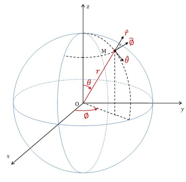
아래 [그림 1]은 구면좌표계의 개념을 설명하기 위한 그림입니다.

1-1. 위치

직각좌표계에서는 어느 입자가 놓인 곳의 위치 좌표를 ( $x$ , $y$ , $z$ )로 표현합니다.

이와 달리 구면좌표계에서는 입자의 좌표를 ( $r$ , $\theta$ , $\phi$ )로 표현해요. 이 세개의 정보만 있으면 3차원 공간의 어느 지점이던 그 위치를 표현할 수 있어요.

[그림 1]과 같이 $r$ 은 원점으로부터 입자가 있는 곳까지의 거리이고, $\theta$ 는 $z$ 축을 기준으로 경도방향으로 돌아간 각도이며, $\phi$ 는 $x$ 축을 기준으로 위도 방향으로 돌아간 각도를 의미합니다.

1-2. 위치벡터

직각좌표계는 세개의 단위벡터 $\hat{x}$ , $\hat{y}$ , $\hat{z}$ 를 이용해 위치벡터를 $\vec {r} = x \hat {x} + y \hat{y} + z\hat{z}$ 로 표현합니다.

그런데 구면좌표계는 위치벡터를 아래 식 (1-1)과 같이 표현해요.

\tag{1-1} \vec r = r \hat{r}

[그림 1]을 보면 $r$ 은 원점으로부터 $M$ 점까지의 거리이고, $\hat{r}$ 은 위치벡터의 방향을 나타내는 단위벡터에요.

그런데 [그림 1]을 보면 단위벡터가 $\hat{r}$ 뿐만 아니라 $\hat{\theta}$ , $\hat{\phi}$ 도 있다는 것을 알 수 있어요.

그럼 다른 단위벡터는 (1)식에서 왜 활용되지 않았나 하고 궁금할 수 있는데요. 그 이유는 단위벡터 $\hat{r}$ 속에 다른 방향 정보가 함께 녹아 있는 것으로 보면 됩니다.

긴 이야기를 시작하기 전에 일단 용어정리를 먼저 할께요.

$\hat{r}$ 은 중심에서 나가는 단위벡터이므로 지름방향단위벡터라고 부릅니다. 그리고 $\hat{\phi}$ 는 위도의 접선방향을 향하며 $\phi$ 방향 단위벡터라고 해요. 마지막으로 $\hat{\theta}$ 는 경도의 접선방향을 향하며 $\theta$ 방향 단위벡터라고 부르면 됩니다.

1-3. 단위벡터

직교좌표계의 가장 기본은 직각좌표계이죠.

따라서 구면좌표계와 직각좌표계 사이의 변환관계를 알고 있어야 언제든지 구면좌표계를 직각좌표계로 바꿀 수 있을 거에요. 물론 그 반대도 가능하죠.

이제부터 구면좌표계와 직각좌표계 사이의 단위벡터 관계를 알아봐요.

[그림 2] 구면좌표계 단위벡터 <span class="katex-eq" data-katex-display="false">\hat r</span>, <span class="katex-eq" data-katex-display="false">\hat \theta</span>, <span class="katex-eq" data-katex-display="false">\hat \phi</span> — [그림 2] 구면좌표계 단위벡터 $\hat r$ , $\hat \theta$ , $\hat \phi$

위 [그림 2]는 [그림 1]을 조금 변형한건데요. $M$ 점의 위치 ( $r$ , $\theta$ , $\phi$ )가 주어져 있을 때 이를 직각좌표계의 위치 ( $x$ , $y$ , $z$ )로 바꾸고자 한다면 어떻게 해야 할까요?

\tag{1-2} (r,~ \theta,~ \phi) \rightarrow(x,~y,~z)

그림을 보면서 상상해 보세요.

[그림 2]에서 $r\sin \theta$ 는 위쪽에 그려진 보라색 실선입니다. 그 실선을 평행이동해서 아래쪽으로 그대로 내리면 원점과 연결된 보라색 선이 될거에요. 그 선의 길이에 $\cos \phi$ 를 취하면 $x$ 좌표를 구할수 있겠어요.

이번에는 원점과 연결된 보라색 선에 $\sin \phi$ 를 취하면 $y$ 좌표를 구할 수 있을거에요.

그럼 $z$ 좌표는 어떻게 구할 수 있나요? 네 맞아요. $r \cos \theta$ 를 구하면 됩니다.

이를 정리하면 ( $r$ , $\theta$ , $\phi$ ) 정보를 이용해 ( $x$ , $y$ , $z$ )를 구할 수 있습니다.

정리하면 아래와 같아요.

\tag{1-3} \begin{align} &x= r \sin \theta \cos \phi\\ &y = r \sin \theta \sin \phi\\ &z = r \cos \theta \end{align}

반대로 ( $x$ , $y$ , $z$ )로부터 ( $r$ , $\theta$ , $\phi$ )를 구하고자 한다면 다음의 관계를 이용하면 됩니다.

\tag{1-4} \begin{align} &r = \sqrt{x^2 + y^2 + z^2}\\ &\theta = \cos^{-1} {z \over r}\\ &\phi = \tan^{-1} {y \over x} \end{align}

(1-4)식의 첫번째는 피타고라스 정리이며, 두번째는 (1-3)식의 세번째 식에서 도출된 것입니다. 그리고 세번째는 (1-3)식의 두번째 식을 첫번째 식으로 나누면 구할 수 있어요.

[단위벡터 유도]

이번에는 구면좌표계의 단위벡터 $\hat{r}$ , $\hat{\theta}$ , $\hat{\phi}$ 를 직각좌표계의 단위벡터 $\hat{x}$ , $\hat{y}$ , $\hat{z}$ 로 표현해봐요.

다시 한번 더 말씀드리면 이런 변환관계는 좌표계끼리 서로 변환할 필요가 있을 때 언제든지 적용하기 위함이라는 것을 기억하세요.

먼저 구면좌표계의 위치벡터인 (1-1)식을 단위벡터 $\hat r$ 에 대해 표현한 후, (1-3)식을적용하면 다음과 같아요.

\tag{1-5} \begin{align} \hat r = {{\vec r}\over{r}} &= {{x\hat x + y \hat y + \hat z}\over{r}}\\ &={{\cancel{r}\sin \theta \cos \phi \hat x + \cancel{r}\sin \theta \sin \phi \hat y + \cancel {r} \cos \theta \hat z}\over{\cancel r}}\\ &=\sin \theta \cos \phi \hat x + \sin \theta \sin \phi \hat y + \cos \theta \hat z \end{align}

이번에는 $\hat \theta$ 를 구해볼텐데요. 이것은 머리속에서 상상을 좀 하셔야 합니다.

[그림 2]에서 $\theta$ 가 현재 그림보다 $\pi \over 2$ 만큼 더 회전하여 $\theta + {\pi \over 2}$ 가 되었다고 상상해 보세요. 그러면 현재 그림의 $\hat r$ 방향이 $\hat \theta$ 의 방향과 같아질거에요. 대신 $\phi$ 는 고정되어 있다는 전제입니다.

이와 같이 $\hat \theta$ 는 $\hat r$ 을 $\theta$ 방향으로 $\pi \over 2$ 만큼 더 회전시키면 구할 수 있는데요. (1-5)식의 단위벡터 $\hat r$ 에 이 관계를 대입하면 다음과 같아요.

\tag{1-6} \begin{align} \hat \theta &= \hat r~~[\theta \rightarrow \theta + {\pi \over 2}, \phi]\\ &=\sin (\theta + {\pi \over 2}) \cos \phi \hat x + \sin (\theta + {\pi \over 2}) \sin \phi \hat y + \cos (\theta + {\pi \over 2}) \hat z\\ &=\cos \theta \cos \phi \hat x + \cos \theta \sin \phi \hat y -\sin \theta \hat z \end{align}

마지막으로 $\hat \phi$ 도 구해봐요. 한번 더 상상을 해보세요. [그림 2]에서 $\hat r$ 이 있잖아요. 이때 만일 $\theta$ 를 ${{\pi}\over{2}}$ 로 고정하고, $\phi$ 를 $\phi + {{\phi}\over{2}}$ 만큼 회전하면 $\hat r$ 이 $\hat \phi$ 과 같아지게 될까요?

네 같은 방향을 향하게 됩니다. 이 관계를 식으로 정리하면 다음과 같아요.

\tag{1-7} \begin{align} \hat \phi &= \hat r~~[\theta = {{\pi}\over{2}},~ \phi \rightarrow \phi + {\pi \over 2}]\\ &=\sin {\pi \over{2}} \cos(\phi + {\pi \over 2}) \hat x + \sin{\pi \over 2} \sin(\phi + {\phi \over 2})\hat y + \cos{\pi \over 2} \hat z\\ &=-\sin \phi \hat x + \cos \phi \hat y \end{align}

최종적으로 (1-5), (1-6), (1-7)식을 종합 정리하면 구면좌표계의 단위벡터는 다음과 같습니다.

\tag{1-8} \begin{align} & \hat r =\sin \theta \cos \phi \hat x + \sin \theta \sin \phi \hat y + \cos \theta \hat z\\ & \hat \theta =\cos \theta \cos \phi \hat x + \cos \theta \sin \phi \hat y -\sin \theta \hat z\\ & \hat \phi = -\sin \phi \hat x + \cos \phi \hat y \end{align}

2. 구면좌표계 속도, 가속도

구면좌표계에서 어느 입자가 있는 곳의 위치벡터는 (1-1)식으로 표현된다고 말씀드렸어요. 그렇다면 구면좌표계에서 그 입자의 속도와 가속도는 어떻게 표현될까요?

이를 구하기 위해서는 우선 (1-8)식에 주어진 구면좌표계 단위벡터를 시간으로 미분하는 것부터 알아야 합니다. 그래야 속도, 가속도 표현을 알아볼 수 있어요.

2-1. 단위벡터의 미분

구면좌표계의 단위벡터는 (1-8)식처럼 총 3개가 있어요. 각각을 시간으로 미분하면 되는데요.

간혹 단위벡터의 크기는 1이고 방향이 각 축의 방향으로 고정되어 있으니 시간으로 미분하면 0이 될것이라고 생각될 수 있어요. 그렇지만 그것은 직각좌표계에서만 맞는 이야기에요. 구면좌표계에서는 0이 아닙니다.

그 이유는 직각좌표계의 단위벡터는 크기가 1이고 방향이 각 축에 고정되어 시간으로 미분하면 0인 것이 맞아요. 하지만 [그림 2]에서 볼수 있는것처럼 구면좌표계의 단위벡터 ( $r$ , $\theta$ , $\phi$ )는 축에 고정된것이 아닙니다.

입자가 있는 위치에 따라 달라져요. 그래서 구면좌표계에서의 단위벡터를 시간으로 미분하면 0이 아닌 것이죠.

그러면 $\hat r$ 부터 시간으로 미분해보겠습니다. 이때 미분을 분수 형태로 써도 좋겠지만 간결하게 표현하기 위해 함수 위에 점을 찍어 표기하겠습니다. 예를 들어 $\theta$ 를 시간 $t$ 로 미분한 ${{d\theta} \over {dt}}$ 를 $\dot \theta$ 처럼요. 그리고 곱의 미분법을 적용합니다.

\tag{2-1} \begin{align} {{{d} \hat r}\over{{d} t}} &= {{d}\over{{d}t}}(\sin \theta \cos \phi \hat x + \sin \theta \sin \phi \hat y + \cos \theta \hat z)\\ &=\cos \theta {{d \theta}\over {dt}}\cos \phi \hat x - \sin \theta \sin \phi {{d \phi}\over{dt}}{\hat x} + \sin \theta \cos \phi {\cancel{{d \hat x}\over{dt}}}\\ &~~~~~~~+\cos {{d \theta}\over{dt}} \sin \phi \hat y + \sin \theta\cos \phi{{d \phi}\over{dt}}\hat y + \sin \theta \sin \phi {\cancel{{d \hat y}\over{dt}}}\\ &~~~~~~~~~~~~~~-\sin \theta {{d \theta}\over{dt}} \hat z + \cos \theta {\cancel{{d \hat z}\over{dt}}}\\ &= \cos \theta\dot \theta\cos \phi \hat x - \sin \theta \sin \phi \dot \phi \hat x + \cos \theta \dot \theta \sin \phi \hat y + \sin \theta \cos \phi \dot \phi \hat y - \sin \theta \dot \theta \hat z\\ &=\dot \theta (\color{blue}{\cos \theta \cos \phi \hat x + \cos \theta \sin \phi \hat y-\sin \theta \hat z}\color{black} ) + \dot \phi \sin \theta(\color{blue}-\sin \phi \hat x + \cos \phi \hat y \color{black})\\ &=\dot \theta \color{blue}\hat \theta \color{black}+\dot \phi \sin \theta \color{blue}\hat \phi \end{align}

위 식에서 사선으로 그어진 항은 직각좌표계 단위벡터를 시간으로 미분한 것이기 때문에 그것은 0이 됩니다.

신기하게도 $\hat r$ 을 시간으로 미분했더니 단위벡터 $\hat \theta$ 와 $\hat \phi$ 의 결합으로 주어지는 것을 알 수 있어요.

이번에는 $\hat \theta$ 를 시간으로 미분해보겠습니다.

\tag{2-2} \begin{align} {{d \hat \theta}\over{dt}} &= {d \over{dt}}(\cos \theta \cos \phi \hat x +\cos \theta \sin \phi \hat y - \sin \theta \hat z)\\ &=-\sin \theta {{d \theta}\over{dt}} \cos \phi \hat x - \cos \theta \sin \phi {{d \phi}\over{dt}}\hat x + \cos \theta \cos \phi {\cancel{{d \hat x}\over{dt}}}\\ &~~~~~~~-\sin \theta {{d \theta}\over{dt}}\sin \phi \hat y + \cos \theta \cos \phi{{d \phi}\over{dt}}\hat y + \cos \theta \sin \phi {\cancel{{d \hat y}\over{dt}}}\\ &~~~~~~~~~~~~~~-\cos \theta {{d \theta}\over{dt}}\hat z - \sin \theta {\cancel{{d \hat z}\over{dt}}}\\ &=- \sin \theta \dot \theta \cos \phi \hat x-\cos \theta \sin \phi \dot \phi\hat x - \sin \theta \dot \theta \sin \phi \hat y+\cos \theta \cos \phi \dot \phi\hat y-\cos \theta \dot \theta \hat z\\ &=\dot \theta (\color{blue}-\sin \theta \cos \phi \hat x-\sin \theta \sin \phi\hat y-\cos \theta \hat z \color{black})+\dot \phi\cos \theta (\color{blue}-\sin \phi \hat x+\cos \phi \hat y \color{black})\\ &=- \dot \theta \color{blue} \hat r \color{black}+ \dot \phi \cos \theta \color{blue}\hat \phi \end{align}

그 결과 단위벡터 $\hat \theta$ 을 시간으로 미분했더니 단위벡터 $\hat r$ 과 $\hat \phi$ 의 결합으로 주어지는 것을 알 수 있어요.

마지막으로 이번에는 $\hat \phi$ 를 시간으로 미분할께요.

\tag{2-3} \begin{align} {{d \hat \phi}\over{dt}} &= {{d}\over{dt}}(-\sin \phi \hat x + \cos \phi \hat y)\\ &=- \cos \phi {{d \phi}\over{dt}}\hat x - \sin \phi {{d \hat x}\over{dt}}-\sin \phi {{d \phi}\over{dt}}\hat y+\cos \phi {{d \hat y}\over{dt}}\\ &=-\cos \phi \dot \phi \hat x - \sin \phi \dot \phi \hat y \end{align}

그 결과 다른 단위벡터와는 달리 $\hat \phi$ 의 시간 미분은 $\hat r$ 과 $\hat \theta$ 의 결합으로 정리되지 않는 것을 알 수 있어요. 뭔가 다른 방법을 시도하면 좋겠는데요.

이렇게 한번 해보겠습니다. $- \hat r$ 에 $\sin \theta \dot \phi$ 를 곱하면 $- \sin \theta \dot \phi \hat r$ 이 됩니다. 그리고 이번에는 $- \theta$ 에 $\cos \theta \dot \phi$ 를 곱하면 $- \cos \theta \dot \phi \hat \theta$ 가 되는데요. 그 두개를 서로 합해봐요.

구체적으로 쓰면 아래와 같습니다.

\tag{2-4} \begin{align} -\sin \theta \dot \phi \hat r+(-\cos \theta \dot \phi \hat \theta)&=-\sin \theta \dot \phi(\sin \theta \cos \phi \hat x + \sin \theta \sin \phi \hat y + \cos \theta \hat z)\\ &~~~~~~~+(-\cos \theta \dot \phi(\cos \theta \cos \phi \hat x + \cos \theta \sin \phi \hat y -\sin \theta \hat z))\\ &=\color{red}-\cos \phi \dot \phi \hat x- \sin \phi \dot \phi \hat y\\ &=\color{blue}{{d \hat \phi}\over{dt}} \end{align}

그 결과 (2-4)식의 빨강색 수식이 (2-3)식의 $\hat \phi$ 을 시간으로 미분한 것과 동일하다는 것을 알 수 있어요. 따라서 $\hat \phi$ 를 시간 미분한 결과는 다음과 같이 쓸 수 있습니다.

\tag{2-5} {{d \hat \phi}\over{dt}} = -\sin \theta \dot \phi \hat r-\cos \theta \dot \phi \hat \theta

구면좌표계 단위벡터 미분에 관한 (2-2), (2-3), (2-5)식을 종합 정리하면 아래 (2-6)식과 같습니다.

\tag{2-6} \begin{align} &{{d \hat r}\over{dt}}= \dot {\hat r}= \dot \theta \color{black}\hat \theta \color{black}+\dot \phi \sin \theta \color{blu}\hat \phi\\ &{{d \hat \theta}\over{dt}} = \dot {\hat \theta}=- \dot \theta \color{ble} \hat r \color{black}+ \dot \phi \cos \theta \color{bue}\hat \phi\\ &{{d \hat \phi}\over{dt}}=\dot {\hat \phi}= -\sin \theta \dot \phi \hat r-\cos \theta \dot \phi \hat \theta \end{align}

2-2. 구면좌표계 속도, 가속도

그럼 이제부터 움직이는 어느 입자가 있을 때, 구면좌표계에서 그 입자의 속도 $\vec v$ 와 가속도 $\vec a$ 가 어떻게 표현되는지 알아보겠습니다.

속도는 단위시간당 위치의 변화량으로 정의됩니다. 이 정의를 활용해 구면좌표계에서의 속도 식을 구하면 다음과 같아요.

\tag{2-7} \begin{align} {\vec v} = {{d \vec r}\over{dt}} &= {{d}\over{dt}}(r \hat r)\\ &=\dot r \hat r + r \dot {\hat r}\\ &=\dot r \hat r + r(\dot \theta \color{black}\hat \theta \color{black}+\dot \phi \sin \theta \color{blu}\hat \phi)\\ &=\dot r \hat r + r \dot \theta \hat \theta + r \dot \phi \sin \theta\hat \phi \end{align}

여기서 첫번째 줄에서 두번째 줄로 넘어갈 때 곱의 미분이 적용되었어요. 그리고 두번째 줄에서 세번째 줄어 넘어갈 때에는 (2-6)식을 적용하였습니다.

이번에는 가속도 표현을 구해보겠습니다.

가속도는 단위시간당 속도의 변화량입니다. 그러므로 (2-7)식을 가져와서 활용하면 됩니다.

\tag{2-8} \begin{align} \vec a = {{d \vec v}\over{dt}} &= {{d}\over{dt}} (\dot r \hat r + r \dot \theta \hat \theta + r \dot \phi \sin \theta \hat \phi)\\ &=\ddot r \hat r + \dot r \dot {\hat r} \\ &~~~~~+ \dot r \dot \theta \hat \theta + r \ddot \theta \hat \theta +r \dot \theta \dot{\hat \theta} \\ &~~~~~+{ {\dot r} {\dot \phi} \sin \theta \hat \phi} + r \ddot \phi \sin \theta \hat \phi + r \dot \phi \cos \theta \dot \theta \hat \phi + r \dot \phi \sin \theta {\dot{\hat \phi}}\\ &=\ddot r \hat r + \dot r ( \dot \theta \color{black}\hat \theta \color{black}+\dot \phi \sin \theta \color{blu}\hat \phi)\\ &~~~~~~+\dot r \dot \theta \hat \theta + r \ddot \theta \hat \theta +r \dot \theta (- \dot \theta \color{ble} \hat r \color{black}+ \dot \phi \cos \theta \color{bue}\hat \phi)\\ &~~~~~~+{ {\dot r} {\dot \phi} \sin \theta \hat \phi} + r \ddot \phi \sin \theta \hat \phi + r \dot \phi \cos \theta \dot \theta \hat \phi + r \dot \phi \sin \theta (-\sin \theta \dot \phi \hat r-\cos \theta \dot \phi \hat \theta)\\ &=(\ddot r - r \dot \phi^2 \sin^2 \theta-r \dot \theta^2) \hat r\\ &~~~~~~+(r \ddot \theta + 2 \dot r \dot \theta - r \dot \phi^2 \sin \theta \cos \theta)\hat \theta\\ &~~~~~~+(r \ddot \phi \sin \theta + 2 \dot r \dot \phi \sin \theta + 2r \dot \theta \dot \phi \cos \theta)\hat \phi \end{align}

3. 미소 길이, 면적, 부피요소

다음은 구면좌표계에서의 미소 길이 요소, 미소 면적 요소, 미소 부피 요소가 어떻게 표현되는지 알아보겠습니다. 우선 미소 길이 요소부터 시작할께요.

3-1. 미소 길이 요소

구면좌표계 위치벡터는 (1)식과 같이 $\vec r = r \hat r$ 로 주어집니다. 이것의 미분을 구하면 그것이 미소 길이 요소 $d \vec r$ 입니다.

그런데 길이 요소를 구하는 것이므로 기호가 $r$ 보다는 $l$ 이 더 친근할 거에요. 그래서 $l$ 로 표기할께요.

\tag{3-1} \begin{align} \vec l &= \vec r = r \hat r\\ d \vec l &= dr \hat r + r d\hat r\\ &=dr \hat r + r\color{red}\Big({{\partial \hat r}\over{\partial \theta}} d \theta + {{\partial \hat r}\over{\partial \phi}} d \phi\Big)\\ &=dr \hat r + r\Big({{\partial}\over{\partial \theta}}(\sin \theta \cos \phi \hat x + \sin \theta \sin \phi \hat y + \cos \theta \hat z)d\theta\\ &~~~~~~~~~~~~~~~~~~~~~+ {{\partial}\over{\partial \phi}}(\sin \theta \cos \phi \hat x + \sin \theta \sin \phi \hat y + \cos \theta \hat z)d \phi\Big)\\ &=dr \hat r + r \Big(\color{blue}(\cos \theta \cos \phi \hat x + \cos \theta \sin \phi \hat y -\sin \theta\hat z)\color{black}d\theta\\ &~~~~~~~~~~~~~~~~~~~~~+ \color{blue}(\sin \theta (- \sin \phi) \hat x + \sin \theta \cos \phi \hat y )\color{black}d \phi \Big)\\ &=dr \hat r + r d \theta \hat \theta + r \sin \theta d \phi\hat \phi\\ &= dl_r \hat r + dl_\theta \hat \theta + dl_\phi \hat \phi \end{align}

(3-1)식의 두번째 줄은 곱의 미분법을 적용한거에요. 그리고 빨강색 수식 부분은 (1-8)식처럼 $\hat r$ 이 $\theta$ 와 $\phi$ 의 함수이므로 $d \hat r$ 을 편미분으로 나타낸거에요. 또한 파랑색 수식 부분은(1-8)식에 주어진 단위벡터 $\hat \theta$ 와 $\hat \phi$ 와 같다는 것을 알 수 있어요.

결국 구면좌표계에서 각 단위벡터 방향의 미소 길이 요소는 다음과 같이 정리할 수 있습니다.

\tag{3-2} \begin{align} &dl_r = dr\\ &d l_\theta = rd\theta\\ &dl_\phi = r \sin \theta d \phi \end{align}

3-2. 미소 면적 요소

이번에는 미소 면적 요소입니다. 아래 [그림 3]을 보아 주세요.

구면에 아주 작은 면적요소가 있는데요. 이 면적요소의 크기는 가로와 세로의 곱으로 주어질 텐데요. 가로를 $\hat \phi$ 방향의 미소 길이 $dl_\phi$ 로 한다면 세로는 $\hat \theta$ 방향의 미소 길이 $dl_\theta$ 가 될거에요.

그래서 미소 면적의 크기는 $dl_\phi$ 와 $dl_\theta$ 의 곱이 됩니다

또한 미소 면적의 방향은 그 면적에 수직한 방향인 단위 벡터 $\hat r$ 으로 설정하면 됩니다.

이것을 정리하면 미소 면적 요소 $d \vec a$ 는 아래와 같이 표현할 수 있어요.

\tag{3-3} \begin{align} d\vec a &= dl_\theta d l_\phi \hat r\\ &=(rd\theta)(r \sin \theta d\phi)\hat r\\ &=r^2 \sin \theta d\theta d\phi \hat r \end{align}

3-3. 미소 부피 요소

구면좌표계의 미소 부피 요소는 위에서 도출한 미소 면적 요소에 미소 높이만 곱해주면 되는데요. 아래 [그림 4]를 보세요.

그림과 같이 높이 요소는 $\hat r$ 방향의 미소 길이 요소인 $dl_r$ 를 적용하면 되겠군요. 이를 정리하면 미소 부피 요소 $d \tau$ 는 다음과 같습니다.

\tag{3-4} \begin{align} d \tau &= dl_r dl_\theta dl_\phi\\ &=(dr)(r d\theta)(r \sin \theta d \phi)\\ &=r^2 \sin \theta dr d\theta d\phi \end{align}

[예제1: 구의 표면적]

구면좌표계에서의 미소 면적 요소를 이용해 반지름이 $r$ 인 구의 표면적을 구하여라.

(Sol) 구면좌표계의 미소 면적을 구의 전체 표면적이 얻어지도록 적분하면 됩니다. 이때 $\theta$ 는 0에서부터 $\pi$ 까지, $\phi$ 는 0에서부터 $2\pi$ 까지 적분합니다.

구체적인 풀이는 다음과 같아요.

\tag{ex-1} \begin{align} S(r) &= \int da\\ &=\int_0^{2\pi}\int_0^{\pi} r^2 \sin \theta d \theta d\phi\\ &=r^2 \int_0^{2\pi} \color{blue} \int_0^{\pi} \sin \theta d \theta \color{black}d\phi\\ &=r^2\int_0^{2\pi} \color{blue}\Big [-\cos \theta \Big]_0^{\pi} \color{black}d \phi\\ &=r^2 \int_0^{2\pi} \color{blue}(1+1) \color{black}d\phi\\ &=2r^2 \int_0^{2\pi} d \phi\\ &=2r^2 \Big [ \phi \Big]_0^{2\pi}\\ &=2r^2(2 \pi - 0)\\ &=4 \pi r^2 \end{align}

우리가 익히 알고 있는 구의 표면적에 관한 식이 도출되었습니다.

[예제2: 구의 부피]

구면좌표계에서의 미소 부피 요소를 이용해 반지름이 $r$ 인 구의 전체 부피를 구하여라.

(Sol) 구면좌표계의 미소 부피를 구의 전체 부피가 얻어지도록 적분하면 됩니다. 이때 $\theta$ 는 0에서부터 $\pi$ 까지, $\phi$ 는 0에서부터 $2\pi$ 까지 적분합니다.

또한 이 경우에는 $r$ 도 0에서부터 $r$ 까지 적분합니다. 그래야 전체 부피가 나오겠죠.

구체적인 풀이는 아래와 같습니다.

\tag{ex-2} \begin{align} V(r) &= \int d \tau\\ &=\int_0^{2 \pi} \int_0^{\pi} \int_0^r r^2 dr \sin \theta d\theta d\phi\\ &=\int_0^{2 \pi} \int_0^{\pi}\Big[{{r^3}\over{3}} \Big]_0^r \sin \theta d\theta d\phi\\ &=\int_0^{2\pi} \int_0^{\pi}{{r^3}\over{3}} \sin \theta d \theta d\phi\\ &={{r^3}\over{3}} \int_0^{2\pi} \int_0^{\pi} \sin\theta d\theta d \phi\\ &={{r^3}\over{3}} \int_0^{2\pi} \Big [-\cos \theta \Big]_0^{\pi}d \phi\\ &={{r^3}\over{3}} \int_0^{2\pi} 2d\phi\\ &={{2}\over{3}}r^3 \int_0^{2\pi} d\phi\\ &={2 \over 3} r^3 \Big[ \phi\Big]_0^{2\pi}\\ &={4 \over 3} \pi r^3 \end{align}

구의 부피를 구하는 식이 도출되었습니다.

4. 델 연산자, 기울기, 발산, 회전

구면좌표계에서의 델 연산자 정의부터 시작해서 스칼라장의 기울기, 벡터장의 발산과 회전을 유도하는 순으로 설명드리겠습니다.

4-1. 델 연산자

직각좌표계에서 미소 길이 요소와 델 연산자 사이의 대응 관계를 보면 아래와 같습니다.

\tag{4-1} d \vec l = dx \hat x + dy \hat y + dz \hat z~~~\rightarrow~~~\nabla = {{\partial}\over{\partial x}}\hat x + {{\partial}\over{\partial y}}\hat y + {{\partial}\over{\partial z}}\hat z

(4-1)의 대응 관계를 구면좌표계에도 적용하면 다음과 같아요. 위에 있는 (3-1)식을 활용하면 됩니다.

\tag{4-2} d \vec l = d l_r \hat r + dl_\theta \hat \theta + d l_\phi \hat \phi~~~\rightarrow~~~\nabla = {{\partial}\over{\partial l_r}}\hat r + {{\partial}\over{\partial l_\theta}} \hat \theta + {{\partial}\over{\partial l_\phi}}\hat \phi

그러면 (4-2)식의 오른쪽에 있는 델 연산자를 조금만 더 구체적으로 정리해 볼까요. (3-2)식을 (4-2)식의 분모에 대입하면 됩니다. 다만 상미분이 편미분으로 바뀌는 것만 달라져요.

그러면 다음과 같이 구면좌표계에서의 델연산자를 정의할 수 있습니다.

\tag{4-3} \nabla = {{\partial}\over{\partial r}} \hat r + {1 \over r}{{\partial}\over{\partial \theta}} \hat \theta + {1 \over {r \sin \theta}}{{\partial}\over{\partial \phi}}\hat \phi

4-2. 스칼라장의 기울기

어떤 스칼라함수 $T$ 가 있을 때 이 함수의 기울기를 구하기 위해서는 델 연산자에 그 스칼라함수를 적용하면 됩니다.

결과적으로 구면좌표계에서 스칼라장 $T$ 의 기울기 벡터는 다음 공식으로 주어집니다.

\tag{4-4} \begin{align} \nabla T &= \Big({{\partial}\over{\partial r}} \hat r + {1 \over r}{{\partial}\over{\partial \theta}} \hat \theta + {1 \over {r \sin \theta}}{{\partial}\over{\partial \phi}}\hat \phi \Big)T\\[10pt] &={{\partial T}\over{\partial r}}\hat r + {1 \over r}{{\partial T}\over{\partial \theta}}\hat \theta + {{1}\over{r \sin \theta}} {{\partial T}\over{\partial \phi}}\hat \phi \end{align}

4-3. 벡터장의 발산

어떤 벡터장 $\vec A = A_r \hat r + A_\theta \hat \theta + A_\phi \hat \phi$ 가 있을 때 이 벡터장의 발산 정도를 구하기 위해서는 델 연산자와 스칼라곱을 해주면 됩니다.

기본 개념식은 다음과 같습니다.

\tag{4-5} \begin{align} \nabla \cdot \vec A &= \Big({{\partial}\over{\partial r}} \hat r + {1 \over r}{{\partial}\over{\partial \theta}} \hat \theta + {1 \over {r \sin \theta}}{{\partial}\over{\partial \phi}}\hat \phi\Big) \cdot \vec A\\[10pt] &={{\partial \vec A}\over{\partial r}} \cdot\hat r + {1 \over r}{{\partial \vec A}\over{\partial \theta}} \cdot\hat \theta + {1 \over {r \sin \theta}}{{\partial \vec A}\over{\partial \phi}}\cdot\hat \phi\\[10pt] &=\Big ( {{\partial A_r}\over{\partial r}}\hat r+ {{\partial A_\theta}\over{\partial r}}\hat \theta+{{\partial A_\phi}\over{\partial r}} \hat \phi \\[10pt] &~~~~~~~~~~~~~~~~~~~~~~~~~~~~~~~~~~~~~~~~~~+ A_r \color{blue}{{\partial \hat r}\over{\partial r}} \color{black}+ A_\theta \color{blue}{{\partial \hat \theta}\over{\partial r}} \color{black}+ A_\phi \color{blue}{{\partial \hat \phi}\over{\partial r}}\color{black}\Big )\cdot \hat r\\[10pt] &~~~~~+\Big ( {{\partial A_r}\over{\partial \theta}}\hat r+ {{\partial A_\theta}\over{\partial \theta}}\hat \theta+{{\partial A_\phi}\over{\partial \theta}} \hat \phi \\[10pt] &~~~~~~~~~~~~~~~~~~~~~~~~~~~~~~~~~~~~~~~~~~+ A_r \color{blue} {{\partial \hat r}\over{\partial \theta}} \color{black}+ A_\theta \color{blue}{{\partial \hat \theta}\over{\partial \theta}} \color{black}+ A_\phi \color{blue}{{\partial \hat \phi}\over{\partial \theta}}\color{black}\Big )\cdot {{\hat \theta}\over{r}}\\[10pt] &~~~~~+\Big ( {{\partial A_r}\over{\partial \phi}}\hat r+ {{\partial A_\theta}\over{\partial \phi}}\hat \theta+{{\partial A_\phi}\over{\partial \phi}} \hat \phi \\[10pt] &~~~~~~~~~~~~~~~~~~~~~~~~~~~~~~~~~~~~~~~~~~+ A_r \color{blue}{{\partial \hat r}\over{\partial \phi}} \color{black}+ A_\theta \color{blue}{{\partial \hat \theta}\over{\partial \phi}} \color{black}+ A_\phi \color{blue}{{\partial \hat \phi}\over{\partial \phi}}\color{black}\Big )\cdot {{\hat \phi}\over{r \sin \theta}}\\[10pt] \end{align}

(4-5)식에서 파랑색으로 표기한 것처럼 단위벡터가 미분되는 부분들이 있는데요. 그 각각의 부분들은 (1-8)식의 단위벡터를 적용하여 구하면 아래와 같습니다.

\tag{4-6} \begin{align} &{{\partial \hat r}\over{\partial r}} = {{\partial}\over{\partial r }}(\sin \theta \cos \phi \hat x + \sin \theta \sin \phi \hat y + \cos \theta \hat z) = 0\\[10pt] &{{\partial \hat \theta}\over{\partial r}} = {{\partial}\over{\partial r }}(\cos \theta \cos \phi \hat x + \cos \theta \sin \phi \hat y -\sin \theta \hat z) = 0\\[10pt] &{{\partial \hat \phi}\over{\partial r}} = {{\partial}\over{\partial r }}(-\sin \phi \hat x + \cos \phi \hat y ) = 0\\[10pt] \newline &{{\partial \hat r}\over{\partial \theta}} = {{\partial}\over{\partial \theta}} (\sin \theta \cos \phi \hat x + \sin \theta \sin \phi \hat y + \cos \theta \hat z) \\ &~~~~~~~~~~~~~~~~~~~~~~~~~~~= \cos \theta \cos \phi \hat x + \cos \theta \sin \phi \hat y -\sin \theta \hat z = \hat \theta\\ &{{\partial \hat \theta}\over{\partial \theta}}={{\partial}\over{\partial \theta}} (\cos \theta \cos \phi \hat x + \cos \theta \sin \phi \hat y -\sin \theta \hat z)\\ &~~~~~~~~~~~~~~~~~~~~~~~~~~~=-(\sin \theta \cos \phi \hat x + \sin \theta \sin \phi \hat y + \cos \theta \hat z) = -\hat r\\ &{{\partial \hat \phi}\over{\partial \theta}}={{\partial}\over{\partial \theta}}(-\sin \phi \hat x + \cos \phi \hat y )=0\\[10pt] \newline &{{\partial \hat r}\over{\partial \phi}} = {{\partial}\over{\partial \phi}}(\sin \theta \cos \phi \hat x + \sin \theta \sin \phi \hat y + \cos \theta \hat z)\\ &~~~~~~~~~~~~~~~~~~~~~~~~~~~=\sin \theta(-\sin \phi \hat x + \cos \phi \hat y )=\sin \theta \hat \phi\\ &{{\partial \hat \theta}\over{\partial \phi}}={{\partial}\over{\partial \phi}}(\cos \theta \cos \phi \hat x + \cos \theta \sin \phi \hat y -\sin \theta \hat z)\\ &~~~~~~~~~~~~~~~~~~~~~~~~~~~=\cos \theta(-\sin \phi \hat x + \cos \phi \hat y )=\cos \theta \hat \phi\\ &{{\partial \hat \phi}\over{\partial \phi}} = {{\partial}\over{\partial \phi}}(-\sin \phi \hat x + \cos \phi \hat y )\\ &~~~~~~~~~~~~~~~~~~~~~~~~~~~=-\cos \phi \hat x - \sin \phi \hat y=-(\sin \theta \hat r+\cos \theta \hat \theta ) \end{align}

위 (4-6)식에서 마지막 줄의 가장 우변을 전개해보면 좌변과 동일한 결과를 얻게 됩니다. 그럼 (4-6)식을 (4-5)식에 대입하겠습니다.

\tag{4-7} \begin{align} \nabla \cdot \vec A &= \Big( {{\partial A_r}\over{\partial r}} \hat r + {{\partial A_\theta}\over{\partial r}} \hat \theta + {{\partial A_\phi}\over{\partial r}} \Big)\cdot \hat r\\[10pt] &~~~~~~ + \Big( {{\partial A_r}\over{\partial \theta}}\hat r + {{\partial A_\theta}\over{\partial \theta}}\hat \theta +{{\partial A_\phi}\over{\partial \theta}}\hat \phi + A_r \hat \theta - A_\theta \hat r \Big) \cdot {{\hat \theta}\over{r}}\\[10pt] &~~~~~~ + \Big({{\partial A_r}\over{\partial \phi}}\hat r + {{\partial A_\theta}\over{\partial \phi}}\hat \theta + {{\partial A_\phi}\over{\partial \phi}}\hat \phi \\[10pt] &~~~~~~~~~~~~~~~~~~~~~~~~~~+A_r \sin \theta \hat \phi+A_\theta \cos \theta \hat \phi +A_\phi[-(\sin \theta \hat r+\cos \theta \hat \theta)] \Big)\cdot{{\hat \phi}\over{r \sin \theta}}\\[10pt] &={{\partial A_r}\over{\partial r}} + {1 \over r} \Big( {{\partial A_\theta}\over{\partial \theta }}+A_r \Big)+{{1}\over{r \sin \theta}} \Big({{\partial A_\phi}\over{\partial \phi}}+A_r \sin \theta +A_\theta \cos \theta \Big) \end{align}

이 과정에서 단위벡터끼리의 스칼라 곱을 연산해야 하는데요. 평행한 성분끼리의 스칼라 곱은 1이되고 수직한 성분끼리의 스칼라 곱은 0이 됩니다.

이제 (4-7)식의 마지막 줄을 최종적으로 정리하면 구면좌표계에서 벡터장의 발산에 대한 식을 도출할 수 있습니다. 아래에 있는 식을 전개해 보면 (4-7)식의 가장 마지막 줄과 같은 식을 얻게 됩니다.

\tag{4-8} \nabla \cdot \vec A = {{1}\over{r^2} }{{\partial}\over{\partial r}}(r^2 A_r) + {1 \over{r \sin \theta}} {{\partial}\over{\partial \theta}}(A_\theta \sin \theta) + {1 \over{r \sin \theta}} {{\partial A_\phi}\over{\partial \phi}}

4-4. 벡터장의 회전

어떤 벡터장 $\vec A = A_r \hat r + A_\theta \hat \theta + A_\phi \hat \phi$ 가 있을 때 이 벡터장의 회전 정도를 구하는 방법입니다. 델 연산자와 벡터장 사이에 벡터곱이 적용되므로 결과는 벡터가 됩니다.

기본 개념식은 다음과 같습니다.

\tag{4-9} \begin{align} \nabla \times\vec A &= \Big({{\partial}\over{\partial r}} \hat r + {1 \over r}{{\partial}\over{\partial \theta}} \hat \theta + {1 \over {r \sin \theta}}{{\partial}\over{\partial \phi}}\hat \phi \Big) \times \vec A\\[10pt] &=\Big(\hat r \times \color{red}{{\partial \vec A}\over{\partial r}}\color{black} \Big)+ \Big({{\hat \theta}\over {r}} \times \color{red}{{\partial \vec A}\over{\partial \theta}} \color{black}\Big) + \Big({{\hat \phi}\over{r \sin \theta}} \times \color{red} {{\partial \vec A}\over{\partial \phi}}\color{black}\Big) \end{align}

그런데 (4-9)식에서 빨강색 수식 부분은 앞에서 (4-5)와 (4-7)식을 통해 이미 계산되었습니다. 따라서 이 계산 결과들이 있는 해당 부분만을 발췌하여 정리하면 아래와 같아요.

\tag{4-10} \begin{align} \nabla \times \vec A &= \Big(\hat r \times \color{red}{{\partial \vec A}\over{\partial r}}\color{black} \Big)+ \Big({{\hat \theta}\over {r}} \times \color{red}{{\partial \vec A}\over{\partial \theta}} \color{black}\Big) + \Big({{\hat \phi}\over{r \sin \theta}} \times \color{red} {{\partial \vec A}\over{\partial \phi}}\color{black}\Big)\\[10pt] &=\hat r \times \Big(\color{red}{{\partial \vec A}\over{\partial r}}\color{black} \Big)+ {{\hat \theta}\over {r}} \times \Big(\color{red}{{\partial \vec A}\over{\partial \theta}} \color{black}\Big) + {{\hat \phi}\over{r \sin \theta}} \times \Big( \color{red} {{\partial \vec A}\over{\partial \phi}}\color{black}\Big)\\[10pt] &= \hat r \times \Big( {{\partial A_r}\over{\partial r}} \hat r + {{\partial A_\theta}\over{\partial r}} \hat \theta + {{\partial A_\phi}\over{\partial r}} \hat \phi \Big)\\[10pt] &~~~~~~~~~+{{\hat \theta}\over{r}} \times \Big( {{\partial A_r}\over{\partial \theta}}\hat r + {{\partial A_\theta}\over{\partial \theta}}\hat \theta +{{\partial A_\phi}\over{\partial \theta}}\hat \phi + A_r \hat \theta - A_\theta \hat r \Big)\\[10pt] &~~~~~~~~~+{{\hat \phi}\over{r \sin \theta}} \times \Big({{\partial A_r}\over{\partial \phi}}\hat r + {{\partial A_\theta}\over{\partial \phi}}\hat \theta + {{\partial A_\phi}\over{\partial \phi}}\hat \phi \\[10pt] &~~~~~~~~~~~~~~~~~~~~~~~~~~+A_r \sin \theta \hat \phi+A_\theta \cos \theta \hat \phi +A_\phi[-(\sin \theta \hat r+\cos \theta \hat \theta)] \Big)\\[10pt] &=\Big({{\partial A_r}\over{\partial r}}(\hat r \times \hat r)+{{\partial A_\theta}\over{\partial r}}(\hat r \times \hat \theta) + {{\partial A_\phi}\over{\partial r}}(\hat r \times \hat \phi)\Big)\\[10pt] &~~~~~~~~~+ {1 \over r}\Big({{\partial A_r}\over{\partial \theta}}(\hat \theta \times \hat r) + {{\partial A_\theta}\over{\partial \theta}}(\hat \theta \times \hat \theta) + {{\partial A_\phi}\over{\partial \theta}}(\hat \theta \times \hat \phi) + A_r(\hat \theta \times \hat \theta) -A_\theta (\hat \theta \times \hat r) \Big)\\[10pt] &~~~~~~~~~+ {1 \over {r \sin \theta}}\Big({{\partial A_r}\over{\partial \phi}}(\hat \phi \times \hat r)+{{\partial A_\theta}\over{\partial \phi}} (\hat \phi \times \hat \theta) + {{\partial A_\phi}\over{\partial \phi}} (\hat \phi \times \hat \phi) \\[10pt] &~~~~~~~~~~~~~~~~~~~~~~~~~~+A_r \sin \theta(\hat \phi \times \hat \phi)+A_\theta \cos \theta(\hat \phi \times \hat \phi) \\[10pt] &~~~~~~~~~~~~~~~~~~~~~~~~~~~~~~~~~~~~~~+A_\phi[-(\sin\theta(\hat \phi \times \hat r)+\cos \theta(\hat \phi \times \hat \theta)] \Big) \end{align}

(4-10)식에는 단위벡터끼리의 벡터곱이 나오는데요. 그것을 순서대로 정리하면 아래와 같습니다.

\tag{4-11} \begin{align} &\hat r \times \hat r = 0\\ &\hat r \times \hat \theta = \hat \phi\\ &\hat r \times \hat \phi = -\hat \theta\\ &\hat \theta \times \hat r = -\hat \phi\\ &\hat \theta \times \hat \theta = 0\\ &\hat \theta \times \hat \phi = \hat r\\ &\hat \phi \times \hat r = \hat \theta\\ &\hat \phi \times \hat \theta = -\hat r\\ & \hat \phi \times \hat \phi = 0 \\ \end{align}

(4-11)식을 (4-10)식에 대입하고 정리해볼께요.

\tag{4-12} \begin{align} \nabla \times \vec A &= \Big( {{\partial A_\theta}\over{\partial r}}\hat \phi - {{\partial A_\phi}\over{\partial r}} \hat \theta\Big)\\[10pt] &~~~~~~~~+{1 \over r} \Big( -{{\partial A_r}\over{\partial \theta}}\hat \phi + {{\partial A_\phi}\over{\partial \theta}}\hat r + A_\theta \hat \phi \Big)\\[10pt] &~~~~~~~~+{{1}\over{r \sin \theta}}\Big( {{\partial A_r}\over{\partial \phi}}\hat \theta - {{\partial A_\theta}\over{\partial \phi}}\hat r + A_\phi [-(\sin \theta \hat \theta-\cos \theta \hat r)] \Big) \end{align}

이제 마지막으로 (4-12)식을 같은 단위벡터끼리 묶어 정리하면 다음의 식을 얻습니다.

\tag{4-13} \begin{align} \nabla \times \vec A &= {{1\over{r \sin \theta}}}\Big[ {{\partial (A_\phi \sin \theta)}\over{\partial \theta}} -{{\partial A_\theta}\over{\partial \phi}} \Big]\hat r\\[10pt] &~~~~~~~~~+{1 \over {r\sin \theta}}\Big[ {{\partial A_r}\over{\partial \phi}}-\sin \theta {{\partial (r A_\phi)}\over{\partial r}} \Big]\hat \theta\\[10pt] &~~~~~~~~~~~~~~~~~~~+{1 \over r}\Big[ {{\partial (r A_\theta)}\over{\partial r}}-{{\partial A_r}\over{\partial \theta}} \Big]\hat \phi \end{align}

벡터곱은 행렬형태로도 표현할 수 있는데요. (4-13)식을 행렬 형태로 표현하면 다음과 같습니다.

\tag{4-14} \begin{align} \nabla \times \vec A = {1 \over{r^2 \sin \theta}} \begin{vmatrix} \hat r & r \hat \theta & r \sin \theta \hat \phi\\ {{\partial}\over{\partial r}} & {{\partial}\over{\partial \theta}} & {{\partial}\over{\partial \phi}}\\A_r & A_\theta & A_\phi \end{vmatrix} \end{align}

4-5. 라플라시안

라플라시안은 어떤 스칼라 함수의 기울기에 대한 발산을 말하는데요. 전자기학 등에서 많이 사용됩니다.

라플라시안은 $\nabla^2$ 으로 표현되는데요. 어떤 스칼라 함수를 $T$ 라고 할 때, 그 함수에 대한 기울기인 (4-3)식과 발산인 (4-4)식을 적용하면 아래와 같이 표현될 수 있습니다.

\tag{4-15} \begin{align} \nabla^2 T &= \nabla \cdot(\nabla T)\\ &= \Big( {{\partial}\over{\partial r}} \hat r + {1 \over r}{{\partial}\over{\partial \theta}} \hat \theta + {1 \over {r \sin \theta}}{{\partial}\over{\partial \phi}}\hat \phi \Big) \cdot \Big({{\partial T}\over{\partial r}}\hat r + {1 \over r}{{\partial T}\over{\partial \theta}}\hat \theta + {{1}\over{r \sin \theta}} {{\partial T}\over{\partial \phi}}\hat \phi\Big)\\ \end{align}

(4-15)식을 한꺼번에 전개하면 아주 복잡하니 하나씩 전개한 후에 합하도록 하겠습니다.

\tag{4-15-1} \begin{align} &{{\partial}\over{\partial r}}\hat r \cdot \Big( {{\partial T}\over{\partial r}}\hat r + {1 \over r }{{\partial T}\over{\partial \theta}} \hat \theta +{1 \over{r \sin \theta}} {{\partial T}\over{\partial \phi}} \hat \phi \Big) \\[10 pt] &~~~~~~~~~~~~=\hat r \cdot\Big[{{\partial}\over{\partial r}}\Big( {{\partial T}\over{\partial r}} \hat r \Big) + {{\partial}\over{\partial r}}\Big( {1 \over r} {{\partial T}\over{\partial \theta}} \hat \theta \Big) + {{\partial}\over{\partial r}} \Big({{1}\over{r \sin \theta}} {{\partial T}\over{\partial \phi}} \hat \phi \Big) \Big]\\[10pt] &~~~~~~~~~~~~=\hat r \cdot\Big[ \Big \{ {{\partial}\over{\partial r}} \Big( {{\partial T}\over{\partial r}} \Big)\hat r+{{\partial T}\over{\partial r}} \color{red}{{\partial \hat r}\over{\partial r}} \color{black} \Big\} + \Big\{ {{\partial}\over{\partial r}} \Big({1 \over r} {{\partial T}\over{\partial \theta}} \Big) \hat \theta+ {1 \over r} {{\partial T}\over{\partial \theta}} \color{red}{{\partial \hat \theta}\over{\partial r}}\color{black} \Big\} \\[10pt] &~~~~~~~~~~~~~~~~~~~~~~~~~~~+ \Big\{ {{\partial}\over{\partial r}} \Big( {1 \over{r \sin \theta}} {{\partial T}\over{\partial \phi}} \Big) \hat \phi + {1 \over{r \sin \theta}}{{\partial T}\over{\partial \phi}} \color{red}{{\partial \hat \phi}\over{\partial r}} \color{black} \Big\} \Big]\\[10pt] &~~~~~~~~~~~~={{\partial }\over{\partial r}} \Big( {{\partial T}\over{\partial r}} \Big) (\hat r \cdot \hat r) + {{\partial}\over{\partial r}} \Big( {1 \over r} {{\partial T}\over{\partial \theta}} \Big) \color{red}(\hat r \cdot \hat \theta) \color{black} + {{\partial}\over{\partial r}} \Big({1 \over{r \sin \theta}} {{\partial T}\over{\partial \phi}}\Big)\color{red}(\hat r \cdot \hat \phi) \\[10 pt] &~~~~~~~~~~~~={{\partial }\over{\partial r}} \Big( {{\partial T}\over{\partial r}} \Big)\\[10pt] &~~~~~~~~~~~~={{\partial^2 T}\over{\partial r^2}} \end{align}

위 (4-15-1)식에서 위로부터 있는 빨강색 수식 3개는 (4-6)식을 적용하면 0이 됩니다. 그리고 아래에 있는 두개의 빨강색 수식은 서로 수직인 단위벡터 사이의 스칼라곱이므로 0이 됩니다.

이번에는 (4-15)식의 두번째 부분을 전개하겠습니다.

\tag{4-15-2} \begin{align} &{1 \over r}{{\partial}\over{\partial \theta}} \hat \theta \cdot \Big({{\partial T}\over{\partial r}} \hat r + {1 \over r} {{\partial T}\over{\partial \theta}} \hat \theta + {1 \over{r \sin \theta}} {{\partial T}\over{\partial \phi}} \hat \phi \Big)\\[10pt] &~~~~~~~~~~~~={{\hat \theta}\over{r}} \cdot \Big[ {{\partial}\over{\partial \theta}} \Big( {{\partial T}\over{\partial r}}\hat r\Big) + {{\partial}\over{\partial \theta}} \Big({{1}\over{r}} {{\partial T}\over{\partial \theta}}\hat \theta\Big) + {{\partial}\over{\partial \theta}}\Big({1 \over{r \sin \theta}}{{\partial T}\over{\partial \phi}}\hat \phi \Big)\Big]\\[10pt] &~~~~~~~~~~~~={{\hat \theta}\over{r}} \cdot \Big[ \Big \{ {{\partial}\over{\partial \theta}}\Big({{\partial T}\over{\partial r}}\Big) \hat r + {{\partial T}\over{\partial r}}\color{blue}{{\partial \hat r}\over{\partial \theta}} \color{black}\Big\} + \Big\{ {{\partial}\over{\partial \theta}}\Big({1 \over r} {{\partial T}\over{\partial \theta}}\Big) \hat \theta + {1 \over r} {{\partial T}\over{\partial \theta}}\color{blue}{{\partial \hat \theta}\over{\partial \theta}} \color{black}\Big\} \\[10pt] &~~~~~~~~~~~~~~~~~~~~~~~~~~~+ \Big\{{{\partial}\over{\partial \theta}} \Big( {1 \over{r \sin \theta}} {{\partial T}\over{\partial \phi}} \Big)\hat \phi + {1 \over{r \sin \theta}} {{\partial T}\over{\partial \phi}}\color{red}{{\partial \hat \phi }\over{\partial \theta}}\color{black} \Big\} \Big]\\[10pt] &~~~~~~~~~~~~=\Big\{{1 \over r}{{\partial }\over{\partial \theta}}\Big({{\partial T}\over{\partial r}}\Big)\color{red}(\hat \theta \cdot \hat r)\color{black} + {1 \over r} {{\partial T}\over{\partial r}}(\hat \theta \cdot \color{blue}\hat \theta \color{black})\Big\} +\Big\{ {1 \over r} {{\partial}\over{\partial \theta}} \Big({1 \over r}{{\partial T}\over{\partial \theta}}\Big) (\hat \theta \cdot \hat \theta) \\[10pt] &~~~~~~~~~~~~~~~~~~~~~~~~~~~+ {1 \over{r^2}} {{\partial T}\over{\partial \theta}}\color{red}(\hat \theta \cdot(-\hat r)) \color{black}\Big\} + \Big\{ {{1}\over{r}}{{\partial}\over{\partial \theta}} \Big({1 \over{r \sin \theta}} {{\partial T}\over{\partial \phi}}\Big)\color{red}(\hat \theta \cdot \hat \phi) \color{black} \Big\} \\[10pt] &~~~~~~~~~~~~={1 \over r} {{\partial T}\over{\partial r}} + {1 \over r^2} {{\partial}\over{\partial \theta}}\Big({{\partial T}\over{\partial \theta}}\Big)\\[10pt] &~~~~~~~~~~~~={1 \over r}{{\partial T}\over{\partial r}} + {1 \over r^2}{{\partial^2 T}\over{\partial \theta^2}} \end{align}

위 (4-15-2)식에서 위로부터 파랑색 수식 2개는 0이 아닙니다. (4-6)식을 적용하면 $\hat \theta$ 과 $- \hat r$ 로 바뀝니다. 그리고 아래 부분에 있는 빨강색 부분은 서로 수직인 단위벡터 사이의 스칼라곱이므로 모두 0이 됩니다.

마지막으로 (4-15)식의 세번째 부분을 전개합니다.

\tag{4-15-3} \begin{align} &{1 \over{r \sin \theta}} {{\partial}\over{\partial \phi}}\hat \phi \cdot \Big( {{\partial T}\over{\partial r}} \hat r + {1 \over r} {{\partial T}\over{\partial \theta}} \hat \theta + {1 \over{r \sin \theta}{{}\over{}}}{{\partial T}\over{\partial \phi}} \hat \phi \Big)\\[10pt] &~~~~~~~~~~~~={\hat \phi \over{r \sin \theta}} \cdot \Big[ {{\partial}\over{\partial \phi}}\Big({{\partial T}\over{\partial r}} \hat r \Big) + {{\partial}\over{\partial{\phi}}}\Big({1 \over r }{{\partial T}\over{\partial \theta}}\hat \theta\Big) + {{\partial}\over{\partial \phi}}\Big({1 \over {r\sin \theta}}{{\partial T}\over{\partial \phi}} \hat \phi \Big)\Big]\\[10pt] &~~~~~~~~~~~~={{\hat \phi}\over{r \sin \theta}} \cdot \Big[ \Big\{ {{\partial}\over{\partial \phi}}\Big( {{\partial T}\over{\partial r}}\Big) \hat r + {{\partial T}\over{\partial r}}\color{blue}{{\partial \hat r}\over{\partial \phi}} \color{black}\Big\} + \Big\{{{\partial}\over{\partial \phi}}\Big( {1 \over r} {{\partial T}\over{\partial \theta}}\Big) \hat \theta + {1 \over r} {{\partial T}\over{\partial \theta}}\color{blue}{{\partial \hat \theta}\over{\partial \phi}}\color{black} \Big\}\\[10pt] &~~~~~~~~~~~~~~~~~~~~~~~~~~~+\Big\{ {{\partial}\over{\partial \phi}}\Big({1 \over{r \sin \theta}}{{\partial T}\over{\partial \phi}}\Big) \hat \phi + {1 \over{r \sin \theta}} {{\partial T}\over{\partial \phi}}\color{blue}{{\partial \hat \phi}\over{\partial \phi}}\color{black} \Big\}\Big]\\[10pt] &~~~~~~~~~~~~=\Big\{{1 \over{r \sin \theta}} {{\partial}\over{\partial \phi}}\Big({{\partial T}\over{\partial r}}\Big)\color{red}(\hat \phi \cdot \hat r)\color{black} + {1 \over{r \sin \theta}} {{\partial T}\over{\partial r}} (\hat \phi \cdot \sin\theta\hat \phi) \Big\} \\[10pt] &~~~~~~~~~~~~~~~~~~~~~~~~~~~+ \Big\{ {1 \over{r \sin \theta}} {{\partial}\over{\partial \phi}}\Big({1 \over r} {{\partial T}\over{\partial \theta}}\Big)\color{red}(\hat \phi \cdot \hat \theta)\color{black}+{1 \over{r\sin \theta}}{1 \over r} {{\partial T}\over{\partial \theta}}(\hat \phi \cdot \cos \theta \hat \phi) \Big\} \\[10pt] &~~~~~~~~~~~~~~~~~~~~~~~~~~~+ \Big\{ {1 \over{r \sin \theta}}{{\partial}\over{\partial \phi}}\Big({{1}\over{r \sin \theta}}{{\partial T}\over{\partial \phi}}\Big) (\hat \phi \cdot \hat \phi) + {1 \over{(r\sin\theta)^2}} {{\partial T}\over{\partial \phi}}\color{red}(\hat \phi \cdot[-(\sin \theta \color{red}\hat r \color{red} + \cos \theta \hat \theta)])\\[10pt] &~~~~~~~~~~~~={1 \over r} {{\partial T}\over{\partial r}} + {{1}\over{r^2}}{{\cos \theta}\over{\sin \theta}}{{\partial T}\over{\partial \theta}} + {1 \over{r^2 \sin^2\theta}}{{\partial}\over{\partial \phi}}\Big({{\partial T}\over{\partial \phi}}\Big)\\[10pt] &~~~~~~~~~~~~={1 \over r} {{\partial T}\over{\partial r}} + {{1}\over{r^2}}{{\cos \theta}\over{\sin \theta}}{{\partial T}\over{\partial \theta}} + {1 \over{r^2 \sin^2\theta}}{{\partial^2 T}\over{\partial \phi^2}} \end{align}

위 (4-15-3)식에서 위에서 파랑색 수식 3개는 0이 아닙니다. (4-6)식을 보면 $\sin \theta \hat \phi$ , $\cos \theta \hat \phi$ , $-(\sin \theta \hat r + \cos \theta \hat \theta)$ 로 바뀝니다. 그리고 아래에 있는 빨강색 수식은 서로 수직인 단위벡터 사이의 스칼라곱이므로 모두 0이 됩니다.

이제 전개가 모두 끝났으니 (4-15-1), (4-15-2), (4-15-3)을 서로 합하면 다음과 같습니다.

\tag{4-16} \begin{align} \nabla^2 T &= \nabla \cdot(\nabla T)\\[10pt] &={{\partial^2 T }\over{\partial r^2}} +\Big[{1 \over r} {{\partial T}\over{\partial r}} + {1 \over r^2} {{\partial^2 T}\over{\partial \theta^2}}\Big]\\[10pt] &~~~~~~~~~~+\Big[{1 \over r} {{\partial T}\over{\partial r}} + {{1}\over{r^2}}{{\cos \theta}\over{\sin \theta}}{{\partial T}\over{\partial \theta}} + {1 \over{r^2 \sin^2\theta}}{{\partial^2T}\over{\partial \phi^2}}\Big] \end{align}

그리고 (4-16)식을 변수별로 분리해서 다시 정리하면 구면좌표계에서 스칼라 함수 $T$ 의 라플라시안은 다음과 같습니다.

\tag{4-17} \begin{align} \nabla^2 T &= \nabla \cdot(\nabla T)\\[10pt] &={1 \over r^2} {{\partial}\over{\partial r}}\Big(r^2 {{\partial T}\over{\partial r}}\Big) + {1 \over{r^2 \sin \theta}} {{\partial}\over{\partial \theta}}\Big(\sin \theta {{\partial T}\over{\partial \theta}}\Big) + {1 \over {r^2 \sin^2 \theta}}{{\partial^2 T}\over{\partial \phi^2}} \end{align}

흥미롭고 도움이 되는 글이었나요? 리뷰를 부탁드립니다.

[Total: 6 Average: 4.3]

구면좌표계(spherical coordinate system)